Global climate
 Global climate statistics, such as the global mean temperature, provide good indicators as to how our global climate varies (e.g. see here). However, most people are not directly affected by global climate statistics. They care about the local climate; the temperature, rainfall and wind where they are. When you look at the impacts of a climate change or specific adaptations to a climate change, you often need to know how a global warming will affect the local climate.
Yet, whereas the global climate models (GCMs) tend to describe the global climate statistics reasonably well, they do not provide a representative description of the local climate. Regional climate models (RCMs) do a better job at representing climate on a smaller scale, but their spatial resolution is still fairly coarse compared to how the local climate may vary spatially in regions with complex terrain. This fact is not a general flaw of climate models, but just the climate models’ limitation. I will try to explain why this is below.
Regional climate characteristics
Most GCMs are able to provide a reasonable representation of regional climatic features such as ENSO, the NAO, the Hadley cell, the Trade winds and jets in the atmosphere. They also provide a realistic description of so-called teleconnection patterns, such as wave propagation in the atmosphere and the ocean. These phenomena, however, tend to have fairly large spatial scales, but when you get down to the very local scale, the GCMs are no longer appropriate.
Minimum scale
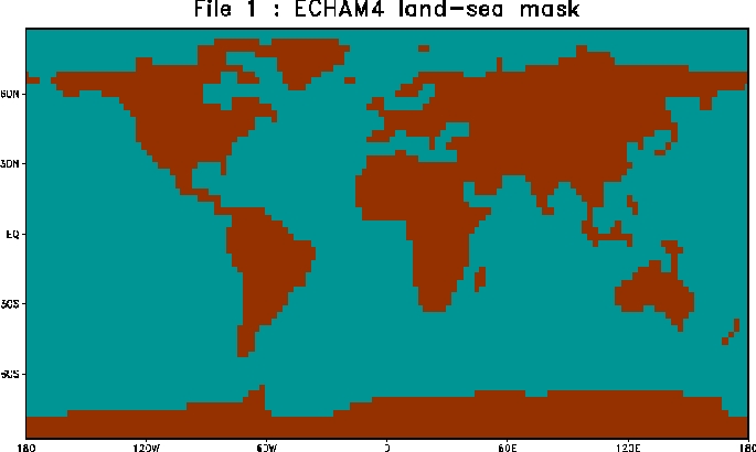 There are several reasons why GCMs do not provide a representative description of the local climate (i.e. exactly where I live). For one, the grid mesh, on which they compute the physical quantities relevant for the climate, is too coarse (typically 200km) to capture the local aspects. The figure on the left shows a typical land-sea mask for a GCM.
The distance between two grid points in a GCM (or an RCM) is the minimum scale (~200km). The coarse resolution typically used in the GCMs till now has implied that the topography has been smooth compared to the real landscape and that some countries (e.g. Denmark and Italy) are not represented in the models (one exception is one Japanese GCM with an extremely high spatial resolution).
Sub-grid processes are represented by parameterisation schemes describing their aggregated effect over a larger scale. These schemes are often referred to as ‘model physics’ but are really based on physics-inspired statistical models describing the mean quantity in the grid box, given relevant input parameters. The parameterisation schemes are usually based on empirical data (e.g. field measurements making in-situ observations), and a typical example of a parameterisation scheme is the representation of clouds.
Surface processes
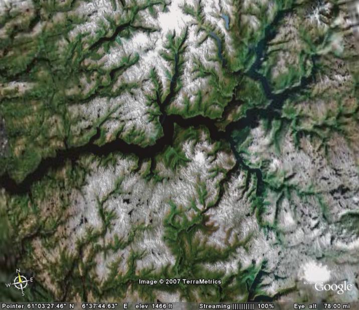 Climate models need boundary conditions describing the surface conditions (e.g. energy and moisture fluxes) in order to yield a realistic representation of the climate system. Often simple parameterisation schemes are employed to provide a reasonable description, but these do not capture the detailed variations associated with small spatial scales.
Skillful scale
Shortcomings associated with parameterisation schemes and coarse resolution explain why one gridpoint value provided by the GCMs may not be representative for the local climate. A concept called skillful scale has sometimes been employed in the literature, most of which have been linked to a study by Grotch and MacCracken (1991) who found model results to diverge as the spatial scale was reduced. Specifically, they observed that:
Although agreement of the average is a necessary condition for model validation, even when [global] averages agree perfectly, in practice, very large regional or pointwise differences can, and do, exist.
Although it is not entirely clear whether this study really touched upon skillful scale, it has since been cited by others, and used to argue that the skillful scale is about 8 gridpoints. Nevertheless, since the 1991-study, the GCMs have improved significantly, and the GCMs now are run for longer periods and with diurnal variations in the insolation.
Regionalisation
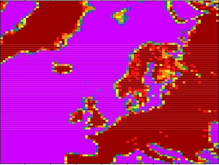
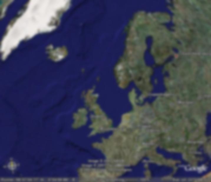
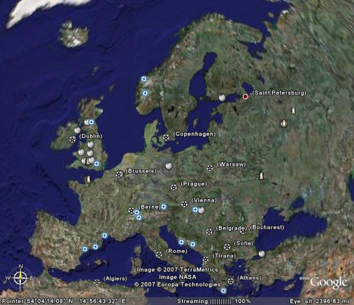
The figure above gives an illustration of the concept of regionalisation, or so-called downscaling. The left panel shows a typical RCM land-sea mask, giving a picture of its spatial resolution. The middle panel shows a blurred satellite image of Europe, which can illustrate how the sharp details are lost yet providing a realistic large-scale picture. The unblurred image of Europe is shown in the right panel. An analogy for the data from GCMs is looking at a blurred picture (middle above) while regional modeling (RCMs) and empirical-statistical downscaling (ESD) is putting on the glasses to improve the image sharpness (right above).
Both RCMs and GCMs give a somewhat ‘blurred’ picture albeit to different degrees of sharpness, and RCMs and GCMs are similar in many respects. However, GCMs are not just ‘blurred’ but also involve some more serious ‘structural differences’ such as an exaggerated Gibraltar Strait (see land-sea mask above), and the Great Lakes area, or Florida, Baja California are quite different and not just blurred (see figure below). Such structural differences are also present in RCMs (eg. fjords), but on much smaller spatial scales.
Yet the images shown here for present climate models do not really show features down to kilometer scales that may influence the local climate where I live, such as valleys, lakes, mountains and fjords, even for RCMs (the lower right panel shows an optimistic projection for improved spatial resolution in GCMs for the near future). The climate in the fjords of Norway (can be be illustrated by the snowcover) is very different from the climate on the mountains separating them. In principle, ESD can be applied to any spatial scale, whereas the RCMs are limited by computer resources and the availability of boundary data.
What is the skilful scale now?
My question is whether the concept of a skillful scale based on old GCMs still apply for the state-of-the-art models. The IPCC AR4 doesn’t say much about skilful scale, but merely states that
Atmosphere-Ocean General Circulation Models cannot provide information at scales finer than their computational grid (typically of the order of 200 km) and processes at the unresolved scales are important. Providing information at finer scales can be achieved through using high resolution in dynamical models or empirical statistical downscaling.
The third assessment report (TAR) merely states that ‘The difficulty of simulating regional climate change is therefore evident’. The IPCC assessment report 4 (chapter 11) and the regionalisation therein will be discussed in a forthcoming post.
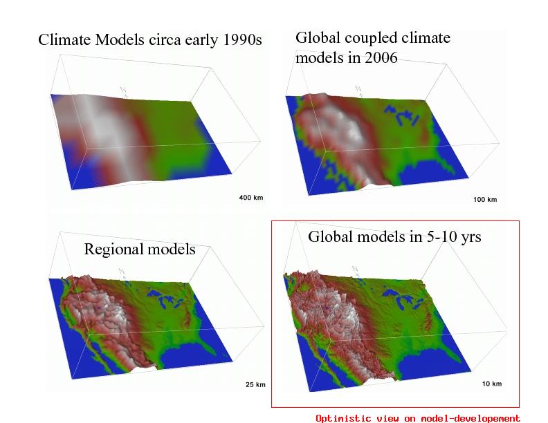 (Source: Strand, NCAR)